Research Article |
|
Corresponding author: Carmelo Maria Musarella ( carmelo.musarella@unirc.it ) Academic editor: Peter de Lange
© 2018 Carmelo Maria Musarella, Ana Cano-Ortiz, José Carlos Piñar Fuentes, Juan Navas-Ureña, Carlos José Pinto Gomes, Ricardo Quinto-Canas, Eusebio Cano, Giovanni Spampinato.
This is an open access article distributed under the terms of the Creative Commons Attribution License (CC BY 4.0), which permits unrestricted use, distribution, and reproduction in any medium, provided the original author and source are credited.
Citation:
Musarella CM, Cano-Ortiz A, Pinar Fuentes JC, Navas-Urena J, Pinto Gomes CJ, Quinto-Canas R, Cano E, Spampinato G (2018) Similarity analysis between species of the genus Quercus L. (Fagaceae) in southern Italy based on the fractal dimension. PhytoKeys 113: 79-95. https://doi.org/10.3897/phytokeys.113.30330
|
Abstract
The fractal dimension (FD) is calculated for seven species of the genus Quercus L. in Calabria region (southern Italy), five of which have a marcescent-deciduous and two a sclerophyllous character. The fractal analysis applied to the leaves reveals different FD values for the two groups. The difference between the means and medians is very small in the case of the marcescent-deciduous group and very large when these differences are established between both groups: all this highlights the distance between the two groups in terms of similarity. Specifically, Q. crenata, which is hybridogenic in origin and whose parental species are Q. cerris and Q. suber, is more closely related to Q. cerris than to Q. suber, as also expressed in the molecular analysis. We consider that, in combination with other morphological, physiological and genetic parameters, the fractal dimension is a useful tool for studying similarities amongst species.
Keywords
deciduous, dimension, fractal analysis, phenotype, sclerophyllous, species, Calabria
Introduction
Quercus L. is an important genus containing several species of trees dominating different forest communities. The ecological and economic role of Quercus spp. is well known (
In the genus Quercus have been counted between 300 (
Leaf morphology has been studied throughout the history of botany, using leaf shape, edge, vein arrangement, hairiness and other features as important characters in systematics (
Numerous authors have noted the comparative inaccuracy of early descriptive and biometric studies (
In their study of several Quercus species,
We calculated the fractal dimension by the box-counting method integrated in the ImageJ software (
The main aim of this work is to establish an analysis of similarity of leaf shape amongst seven species in the genus Quercus from Italy and corroborate our previous studies (
Methods
Data collection
In this work, we analysed 7 species living in Calabria using 275 tree samples belonging to Quercus robur subsp. brutia, Q. cerris, Q. congesta, Q. crenata, Q. ilex subsp. ilex, Q. suber and Q. virgiliana. Orientation largely determines the amount of light the leaves receive for photosynthesis and their size can thus be affected by this greater or lesser exposure to light. For this reason, samples were taken from the four cardinal points on each tree to examine the possible influence of orientation on leaf development. A total of 1,099 leaves were analysed from 120 samples of Q. robur subsp. brutia, 120 from Q. cerris, 154 from Q. congesta, 147 from Q. crenata, 240 from Q. ilex subsp. ilex, 139 from Q. suber and 179 from Q. virgiliana. All the leaves were colour-scanned in a scanner with a resolution of 1200 dpi and 24-bit colour. After scanning, the leaf was transformed to image 8-bit greyscales and the image was segmented by selecting the greyscale between 111 and 126. We opened this image with the ImageJ programme in order to determine its fractal dimension (FD).
The fractal dimension (FD)
Fractal geometry is the most suitable method for characterising the complexity of the vascular system or other mathematically similar structures such as stream drainage networks in chicken embryos or the distribution of the vascular system of a leaf (
All man-made objects can be described in simple shapes using Euclidean geometry. However, natural objects have irregular forms that cannot always be represented using this method (
Due to the recentness of the discovery and its wide range of applications, there is still no universal definition of what actually constitutes a fractal. They are thus described according to their common properties: specifically, they must have the same appearance at any scale of observation, meaning that a fractal object can be broken down into parts, each of which is identical to the whole object (self-affinity or self-similarity); they must have a fractional and not a whole dimension (fractal dimension); and finally the relationship between two of their variables must be a power law (where the exponent is its fractal dimension,
When an object is totally self-similar, such as the mathematical fractal known by the name of the Koch curve (Figure

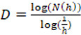
A unit segment can be divided – for example – into three pieces similar to the original, each with a length of 1/3. In general, where N(h) is the number of pieces with a length h, it follows that N(h) ∙ h1 = 1. If we now look at a square with a unit side, we can break it down into 9 = 32 smaller squares with a side of ⅓; that is to say N(h) ∙ h2 = 1. Finally, in the case of a cube, it is easy to see that the following is true: N(h) ∙ h3 = 1. That is, the exponent of h coincides with the topological and Euclidean dimension of the straight line (1), the square (2) and the cube (3) (
By extrapolation from this concept, if the object is completely self-similar, there is a relationship between the scale factor h and the number of pieces N(h) into which the object can be divided, which is given by N(h) = (1/h)D; that is to say
 .
.
Thus the fractal dimension of the Koch curve is:
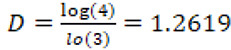 ,
,
a number that is very similar to the FD of the English coastline.
However, natural objects like leaves are not perfect fractals, as they are not totally self-similar but are said to be statistically similar. In this case, the value of their fractal dimension is known by the name of Hausdorff-Besicovitch and is:
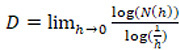 .
.
The calculation of this limit is somewhat complicated and requires the use of different algorithms such as dilation methods, the perimeter method, Grassberger and Procaccia’s correlation dimension and box-counting method. This last is the most widely used as it is very simple to implement with computer technology and highly accurate (
To find the fractal dimension of a digital image using the box-counting method (
| Label | C2 | C3 | C4 | C6 | C8 | C12 | C16 | C32 | D |
| QCONGESTA1_E_01 | 358874 | 166858 | 97125 | 44308 | 25268 | 11452 | 6553 | 1727 | 1.93 |
The graphic representation of the regression line and the point cluster shows two very clearly differentiated parts. The minimum and maximum box size is therefore very important when applying this method. In fact, the approximation error must be reduced by selecting points with a “more linear” form as a box size.
Calculating the fractal dimension (FD)
The FD was calculated by the box-counting method (

The box-counting algorithm was then applied to this black-and-white image of the venation network of the leaf to calculate the FD with box sizes (h) ranging from 2 to 32. Specifically, the image is covered with a grid of squares initially with side 2 and subsequently with squares with sides 3, 4, 6, 8, 12, 16 and 32 (in the image C2, C3, C4, C6, C8, C12, C16 and C32). Table
Once the points were represented (log(1/h), log(N(h)), we calculated the regression line (Figure

For the statistical treatment, the mean FDs were obtained for each species and an analysis of variance was undertaken to test for significant differences amongst the means. First, the Shapiro-Wilk normality test and the difference between the mean, median and kurtosis indicate that our data do not follow a normal distribution (Table
| Taxa | Median | Mean | Variance (n-1) | Kurtosis (Pearson) | St. root of the variance | St. root [kurtosis (Fisher)] | |
|---|---|---|---|---|---|---|---|
| North | Q. robur subsp. brutia | 1.5440 | 1.5290 | 0.0730 | -1.3300 | 0.0192 | 0.8327 |
| Q. cerris | 1.6760 | 1.6676 | 0.0375 | -0.5768 | 0.0098 | 0.8327 | |
| Q. congesta | 1.8780 | 1.8310 | 0.0138 | 1.8836 | 0.0032 | 0.7587 | |
| Q. crenata | 1.9195 | 1.8669 | 0.0172 | 6.2735 | 0.0040 | 0.7497 | |
| Q. ilex subsp. ilex | 1.3530 | 1.3804 | 0.0297 | 0.9245 | 0.0055 | 0.6133 | |
| Q. suber | 0.8620 | 0.9001 | 0.0703 | 0.3360 | 0.0173 | 0.7879 | |
| Q. virgiliana | 1.9310 | 1.9192 | 0.0016 | 7.4011 | 0.0003 | 0.6876 | |
| South | Q. robur subsp. brutia | 1.7675 | 1.6220 | 0.0895 | -1.6597 | 0.0235 | 0.8327 |
| Q. cerris | 1.6600 | 1.6190 | 0.0337 | 0.3597 | 0.0089 | 0.8327 | |
| Q. congesta | 1.9000 | 1.8749 | 0.0058 | 2.8406 | 0.0014 | 0.7587 | |
| Q. crenata | 1.9200 | 1.8803 | 0.0106 | 2.8957 | 0.0025 | 0.7497 | |
| Q. ilex subsp. ilex | 1.3610 | 1.3442 | 0.0149 | -0.2129 | 0.0028 | 0.6133 | |
| Q. suber | 0.9395 | 0.9487 | 0.0408 | 0.0321 | 0.0100 | 0.7879 | |
| Q. virgiliana | 1.9120 | 1.8780 | 0.0060 | 1.1207 | 0.0013 | 0.6876 | |
| East | Q. robur subsp. brutia | 1.8405 | 1.7336 | 0.0428 | -0.2321 | 0.0112 | 0.8327 |
| Q. cerris | 1.8360 | 1.8110 | 0.0143 | -0.0039 | 0.0037 | 0.8327 | |
| Q. congesta | 1.9230 | 1.9215 | 0.0008 | 2.2392 | 0.0002 | 0.7587 | |
| Q. crenata | 1.9270 | 1.8476 | 0.0257 | 1.2883 | 0.0060 | 0.7497 | |
| Q. ilex subsp. ilex | 1.3170 | 1.2954 | 0.0196 | 1.7224 | 0.0036 | 0.6133 | |
| Q. suber | 0.8850 | 0.9059 | 0.0475 | -0.3256 | 0.0117 | 0.7879 | |
| Q. virgiliana | 1.9445 | 1.9287 | 0.0032 | 11.3639 | 0.0007 | 0.6876 | |
| West | Q. robur subsp. brutia | 1.5715 | 1.5676 | 0.0800 | -1.2799 | 0.0210 | 0.8327 |
| Q. cerris | 1.6050 | 1.6116 | 0.0643 | 2.0300 | 0.0169 | 0.8327 | |
| Q. congesta | 1.9180 | 1.8985 | 0.0030 | 0.4157 | 0.0007 | 0.7587 | |
| Q. crenata | 1.9030 | 1.8754 | 0.0085 | 2.8668 | 0.0020 | 0.7497 | |
| Q. ilex subsp. ilex | 1.4170 | 1.4302 | 0.0429 | 0.1534 | 0.0080 | 0.6133 | |
| Q. suber | 0.9535 | 0.9746 | 0.0615 | 0.2308 | 0.0151 | 0.7879 | |
| Q. virgiliana | 1.9440 | 1.9317 | 0.0015 | 6.6553 | 0.0003 | 0.6876 | |
| Mean | Q. robur subsp. brutia | 1.5500 | 1.6130 | 0.0493 | -1.6202 | 0.0129 | 138.47.00 |
| Q. cerris | 1.7029 | 1.6773 | 0.0253 | 1.8675 | 0.0066 | 0.8327 | |
| Q. congesta | 1.8960 | 1.8815 | 0.0026 | -0.6569 | 0.0006 | 0.7587 | |
| Q. crenata | 1.8866 | 1.8675 | 0.0052 | 0.9650 | 0.0012 | 0.7497 | |
| Q. ilex subsp. ilex | 1.3625 | 1.3625 | 0.0053 | -0.4868 | 0.0010 | 0.6133 | |
| Q. suber | 0.9164 | 0.9323 | 0.0267 | -0.1453 | 0.0066 | 0.7879 | |
| Q. virgiliana | 1.9184 | 1.9144 | 0.0007 | -0.9555 | 0.0001 | 0.6876 |
In the hypothetical case that the difference between the fractal values (means and medians) for two species is zero or has a quotient of one, the degree of relationship between the two species is 100%; DfA – DfB = 0; DfA / DfB = 1, species A and B are equal; thus the lower the fractal difference or the nearer the fractal quotient is to 1, the greater the similarity between the species.
Results
The analysis of the FD values for each orientation and for each species shows that for Q. robur subsp. brutia, Q. cerris, Q. congesta and Q. virgiliana, the orientation influences the values of FD, as there are significant differences for these species (Table
Kruskal-Wallis analysis for the values of FD in each orientation for each of the species. In bold: the significant values for which orientation influences the FD at 95% confidence.
| Kruskal-Wallis: | Q. robur subsp. brutia | Q. cerris | Q. congesta | Q. crenata | Q. ilex subsp. ilex | Q. suber | Q. virgiliana |
|---|---|---|---|---|---|---|---|
| Mean North | 1.5290 | 1.6676 | 1.8310 | 1.8669 | 1.3804 | 0.9001 | 1.9192 |
| Mean South | 1.6220 | 1.6190 | 1.8749 | 1.8803 | 1.3442 | 0.9487 | 1.8780 |
| Mean East | 1.7336 | 1.8110 | 1.9215 | 1.8476 | 1.3276 | 0.9059 | 1.9287 |
| Mean West | 1.5676 | 1.6116 | 1.8985 | 1.8754 | 1.3895 | 0.9746 | 1.9317 |
| St. Deviation North | 0.2702 | 0.1936 | 0.1174 | 0.1313 | 0.1723 | 0.2651 | 0.0406 |
| St. Deviation South | 0.2992 | 0.1836 | 0.0763 | 0.1030 | 0.1220 | 0.2020 | 0.0777 |
| St. Deviation East | 0.2069 | 0.1194 | 0.0288 | 0.1602 | 0.1074 | 0.2180 | 0.0563 |
| St. Deviation West | 0.2829 | 0.2535 | 0.0546 | 0.0921 | 0.1564 | 0.2479 | 0.0392 |
| K (Observed value) | 9.9875 | 20.5115 | 23.0332 | 1.6844 | 8.0795 | 3.0683 | 38.4400 |
| K (Critical value) | 9.4877 | 7.8147 | 7.8147 | 7.8147 | 9.4877 | 7.8147 | 7.8147 |
| p-value | 0.0406 | 0.0001 | < 0.0001 | 0.6404 | 0.0887 | 0.3812 | < 0.0001 |
These species correspond to deciduous or marcescent species, whereas the perennial species Q. ilex subsp. ilex, Q. suber and Q. crenata do not show significant differences in the values of FD for the different levels of orientation.
An analysis of the average FD values for each species indicates that there are significant differences between the different levels of species under study (Table
| K (Observed value) | 220.2702 |
| K (Critical value) | 12.5916 |
| GDL | 6 |
| p-value (bilateral) | < 0.0001 |
| alpha | 0.05 |
Differences in FD by pairs between each species (in parentheses, p-value). In bold: significant differences at 95% confidence.
| Q. robur subsp. brutia | Q. cerris | Q. congesta | Q. crenata | Q. ilex subsp. ilex | Q. suber | Q. virgiliana | |
|---|---|---|---|---|---|---|---|
| Q. robur subsp. brutia | – | ||||||
| Q. cerris | 4.26 (0.6392) | – | |||||
| Q. congesta | 71.21 (<0.0001) | 66.95 (<0.0001) | – | ||||
| Q. crenata | 68.55 (<0.0001) | 64.29 (<0.0001) | -2.65 (0.7439) | – | |||
| Q. ilex subsp. ilex | -58.63 (<0.0001) | -62.9 (<0.0001) | -129.85 (<0.0001) | -127.19 (<0.0001) | – | ||
| Q. suber | -109.43 (<0.0001) | -113.7 (<0.0001) | -180.65 (<0.0001) | -177.99 (<0.0001) | -50.8 (<0.0001) | – | |
| Q. virgiliana | 96.87 (<0.0001) | 92.61 (<0.0001) | 25.66 (0.001) | 28.32 (0.0002) | 155.51 (<0.0001) | 206.31 (<0.0001) | – |
As can be seen in Table
The analysis of the medians of the seven groups (Figure

In the multiple comparison analysis (Figure

In the case of both mean and median values, it is confirmed that the value of the fractal dimension (FD) is less than 1.6 in the case of sclerophyllous Quercus and greater for marcescent and deciduous Quercus (Figure
The differences between average FD values for marcescent and deciduous Quercus species are very low (Table
| Species | Count | Sum of the ranges | Mean of the ranges | Homogeneous groups | ||||
|---|---|---|---|---|---|---|---|---|
| Q. suber | 34 | 626.0000 | 18.4118 | A | ||||
| Q. ilex subsp. ilex | 59 | 4083.5000 | 69.2119 | B | ||||
| Q. robur subsp. brutia | 30 | 3835.5000 | 127.8500 | C | ||||
| Q. cerris | 30 | 3963.5000 | 132.1167 | C | ||||
| Q. crenata | 38 | 7463.5000 | 196.4079 | D | ||||
| Q. congesta | 37 | 7365.5000 | 199.0676 | D | ||||
| Q. virgiliana | 46 | 10337.5000 | 224.7283 | E | ||||
Based on the differences obtained from FDA–FDB = 0, the most closely related species are: Q. congesta-Q. crenata 0.023; Q. cerris-Q. robur subsp. brutia 0.064; Q. virgiliana-Q. congesta 0.033; Q. virgiliana-Q. crenata 0.046; and Q. crenata-Q. cerris 0.191. The most distant relationship is between Q. virgiliana-Q. suber 0.982 and Q. congesta-Q. suber 0.949 (Figure
Discussion
There is a widespread consensus that complex objects with the same features can be included in the category of fractals. Self-similarity is one of the characteristics of fractal objects, meaning that when these images are broken down into smaller pieces, each one is identical to the whole. The fractional dimension is another of its features.
In the hypothetical case that the difference between the fractal values of two species is zero, or their quotient is one, the degree of relationship between the two species is 100%: DfA – DfB = 0; DfA / DfB = 1, species A and B are equal. Thus the smaller the fractal difference or the closer the fractal quotient is to 1, the greater the similarity between the species; if the value of this quotient is far from 1, as occurs between Dfvi/Dfsu > 2, the species Q. virgiliana and Q. suber are very distant from each other. This occurs when the fractal values are the same and means that the same or similar characters have been measured
Finally, the orientation has no influence on the fractal dimension between either the same species or between the different species. This means that the shape of the distribution of the leaf vascular network is not affected by possible changes in orientation, thus discounting the effects of environmental variables such as amount of light, temperature, humidity etc., associated with orientation. This evidence is important in Quercus species, as in other cases, these environmental variables can influence seed germination and the capacity of some plant species to adapt to extreme environments (
Conclusions
We confirm that the application of fractal analysis identifies the phenotypical differences between species and can be used as a method to establish their degree of relationship; this is supported by molecular analysis by various authors. In this work we can affirm that sclerophyllous Quercus species have a fractal dimension of < 1.6 and marcescent and deciduous Quercus species have FD > 1.6; and that Q. crenata, a hybrid of Q. suber and Q. cerris, has a greater similarity to Q. cerris than to Q. suber. The low values of the mean and median FD revealed by the differences between the FD for marcescent-deciduous Quercus species suggest a high degree of similarity amongst the five marcescent-deciduous species. Based on their FD, marcescent Quercus species (semideciduous) are more closely related to deciduous than to sclerophyllous Quercus species, whereas the sclerophyllous Q. ilex subsp. ilex and Q. suber show substantial morphological differences with the marcescent and deciduous Quercus species, as evidenced by fractal analysis. These two species have followed different evolutionary paths from the others, as is to be expected, as the centre of origin of sclerophyllous Quercus species is Mediterranean, whereas deciduous Quercus species have a temperate origin and marcescent Quercus species come from the boundary between the Temperate and Mediterranean bioclimates (
Acknowledgements
We are very grateful to the anonymous referees and to Subject Editor Peter de Lange for their suggestions for improving the original article. This article has been translated by Ms Pru Brooke-Turner (M.A. Cantab.), a native English speaker specialising in scientific texts.
References
- AA.VV (2013) Interpretation Manual of European Union Habitats, version EUR 28. European Commission, DG Environment. Nature ENV B.3. https://eunis.eea.europa.eu/references/2435 [accessed 10.11.2018]
- Abramoff MD, Magalhaes PJ, Ram SJ (2004) Image Processing with ImageJ. Biophotonics International 11(7): 36–42.
- Amaral Franco J (1990) Quercus L. In: Castroviejo S (Ed.) Flora Ibérica. Consejo Superior De Investigaciones Cientificas. Madrid, vol. II, 15–36.
- Bartolucci F, Peruzzi L, Galasso G, Albano A, Alessandrini A, Ardenghi NMG, Astuti G, Bacchetta G, Ballelli S, Banfi E, Barberis G, Bernardo L, Bouvet D, Bovio M, Cecchi L, Di Pietro R, Domina G, Fascetti S, Fenu G, Festi F, Foggi B, Gallo L, Gottschlich G, Gubellini L, Iamonico D, Iberite M, Jiménez-Mejías P, Lattanzi E, Marchetti D, Martinetto E, Masin RR, Medagli P, Passalacqua NG, Peccenini S, Pennesi R, Pierini B, Poldini L, Prosser F, Raimondo FM, Roma-Marzio F, Rosati L, Santangelo A, Scoppola A, Scortegagna S, Selvaggi A, Selvi F, Soldano A, Stinca A, Wagensommer RP, Wilhalm T, Conti F (2018) An updated checklist of the vascular flora native to Italy. Plant Biosystems 152(2): 179–303. https://doi.org/10.1080/11263504.2017.1419996
- Biondi E, Blasi C, Burrascano S, Casavecchia S, Copiz R, Del Vico E, Galdenzi D, Gigante D, Lasen C, Spampinato G, Venanzoni R, Zivkovic L (2009) Manuale Italiano di Interpretazione degli habitat della Direttiva 92/43/CEE. SBI, MATTM, DPN. http://vnr.unipg.it/ha- bitat/index.jsp [accessed 10.11.2018]
- Brullo S, Guarino R (2017) Quercus L. In: Pignatti S (Ed.) Flora d’Italia vol.2. Edagricole, Bologna, 686–697.
- Brullo S, Guarino R, Siracusa G (1999) Taxonomical revision about the deciduous oaks of Sicily. Webbia 54(1): 1–72. https://doi.org/10.1080/00837792.1999.10670670
- Brullo S, Scelsi F, Spampinato G (2001) La vegetazione dell’Aspromonte. Studio Fitosociologico. Laruffa Editore, Reggio Calabria, 372 pp.
- Camarero JJ, Sisó S, Gil-Pelegrín E (2003) Fractal Dimension does not adequately describe the complexity of leaf margin in seedlings of Quercus species. Anales del Jardin Botanico de Madrid 60: 63–71. https://doi.org/10.3989/ajbm.2002.v60.i1.82
- Cano E, Musarella CM, Cano-Ortiz A, Piñar Fuentes JC, Spampinato G, Pinto Gomes C (2017) Morphometric analysis and bioclimatic distribution of Glebionis coronaria s.l. (Asteraceae) in the Mediterranean area. PhytoKeys 81: 103–126. https://doi.org/10.3897/phytokeys.81.11995
- Conte L, Cotti C, Cristofolini G (2007) Molecular evidence for hybrid origin of Quercus crenata Lam. (Fagaceae) from Q. cerris L. and Quercus suber L. Plant Biosystems 141(2): 181–193. https://doi.org/10.1080/11263500701401463
- Coutinho AXP (1939) A flora de Portugal (Plantas vasculares) disposta em chaves dichotomicas. Aillaud, Alves & C, Paris, 938 pp.
- Coutinho JP, Carvalho A, Lima-Brito J (2014) Genetic diversity assessment and estimation of phylogenetic relationships among 26 Fagaceae species using ISSRs. Biochemical Systematics and Ecology 54: 247–256. https://doi.org/10.1016/j.bse.2014.02.012
- Coutinho JP, Carvalho A, Lima-Brito J (2015) Taxonomic and ecological discrimination of Fagaceae species based on internal transcribed spacer polymerase chain reaction–restriction fragment length polymorphism. AoB Plants 7: plu079. https://doi.org/10.1093/aobpla/plu079
- Curtu AL, Gailing O, Finkeldey R (2007) Evidence for hybridization and introgression within a species-rich oak (Quercus spp.) community. BMC Evolutionary Biology 7(1): 218. https://doi.org/10.1186/1471-2148-7-218
- Cuzzocrea A, Mumolo E, Grasso GM (2017) Genetic Estimation of Iterated Function Systems for Accurate Fractal Modeling in Pattern Recognition Tools. In: Gervasi O, et al. (Eds) Computational Science and Its Applications – ICCSA 2017. ICCSA 2017. Lecture Notes in Computer Science, vol 10404. Springer, Cham. https://doi.org/10.1007/978-3-319-62392-4_26
- De Araujo Mariath JE, Pires Dos Santos R, Pires Dos Santos R (2010) Fractal dimension of the leaf vascular system of three Relbunium species (Rubiaceae). Brazilian Journal of Biosciences 8(1): 30–33. http://www.ufrgs.br/seerbio/ojs/index.php/rbb/article/view/1247 [accessed 10.10.2018]
- De Paola P, Del Giudice V, Massimo DE, Forte F, Musolino M, Malerba A (2019) Isovalore Maps for the Spatial Analysis of Real Estate Market: A Case Study for a Central Urban Area of Reggio Calabria, Italy. In: Calabrò F, Della Spina L, Bevilacqua C (Eds) New Metropolitan Perspectives.ISHT 2018. Smart Innovation, Systems and Technologies, vol 100, Springer, Cham, 402–410. https://doi.org/10.1007/978-3-319-92099-3_46
- Del Giudice V, Massimo DE, De Paola P, Forte F, Musolino M, Malerba A (2019) Post Carbon City and Real Estate Market: Testing the Dataset of Reggio Calabria Market Using Spline Smoothing Semiparametric Method. In: Calabrò F, Della Spina L, Bevilacqua C (Eds) New Metropolitan Perspectives.ISHT 2018. Smart Innovation, Systems and Technologies, vol 100, Springer, Cham, 206–214. https://doi.org/10.1007/978-3-319-92099-3_25
- Elias TS (1971) The genera of Fagaceae in the southeastern United States. Journal of the Arnold Arboretum 52: 159–195. https://doi.org/10.5962/bhl.part.9112
- Esteban FJ, Sepulcre J, Vélez De Mendizábal N, Goñi J, Navas J, Ruiz De Miras J, Bejarano B, Masdeu JC, Villoslada P (2007) Fractal dimensión and White matter changes in multiple sclerosis. NeuroImage 36(3): 543–549. https://doi.org/10.1016/j.neuroimage.2007.03.057
- Esteban FJ, Sepulcre J, Ruiz De Miras J, Navas J, Vélez De Mendizábal N, Goñi J, Quesada JM, Bejarano B, Villoslada P (2009) Fractal dimensión analysis of grey matter in multiple sclerosis. Journal of the Neurological Sciences 282(1–2): 67–71. https://doi.org/10.1016/j.jns.2008.12.023
- Fortini P, Di Marzio P, Di Pietro R (2015) Differentiation and hybridization of Quercus frainetto, Q. petraea, and Q. pubescens (Fagaceae): Insights from macro-morphological leaf traits and molecular data. Plant Systematics and Evolution 301(1): 375–385. https://doi.org/10.1007/s00606-014-1080-2
- Glenny RW, Robertson HT, Yamashiro S (1985) . Applications of fractal analysis to physiology. Journal of Applied Physiology 70(6): 2351.2367. https://doi.org/10.1152/jappl.1991.70.6.2351
- Hickey LJ (1979) A Revised Classification of the Architecture of Dicotyledonous Leaves. In: Metcalfe CR, Chalk LM (Eds) Anatomy of the Dicotyledons.Clarendon Press, Oxford, 1, 25–39.
- Hickey LJ, Wolfe JA (1975) The bases of Angiosperm phylogeny: Vegetative morphology. Annals of the Missouri Botanical Garden 62(3): 538–589. https://doi.org/10.2307/2395267
- Horton RE (1945) Erosional development of streams and their drainage basins; hydrophysical approach to quantitative morphology. Geological Society of America Bulletin 56(3): 275–370. https://doi.org/10.1130/0016-7606(1945)56[275:EDOSAT]2.0.CO;2
- Lawrence GHM (1951) Taxonomy of Vascular Plants. MacMillan Co., New York, 823 pp.
- Li J, Du Q, Sun C (2009) An improved box-counting method for image fractal dimension estimation. Pattern Recognition 42(11): 2460–2469. https://doi.org/10.1016/j.patcog.2009.03.001
- Lopes R, Beltrouni N (2009) Fractal and multifractal analysis: A review. Medical Image Analysis 13(4): 634–649. https://doi.org/10.1016/j.media.2009.05.003
- Malerba A, Massimo DE, Musolino M, Nicoletti F, De Paola P (2019) Post Carbon City: Building Valuation and Energy Performance Simulation Programs. In: Calabrò F, Della Spina L, Bevilacqua C (Eds) New Metropolitan Perspectives.ISHT 2018. Smart Innovation, Systems and Technologies, vol 101, Springer, Cham, 513–521. https://doi.org/10.1007/978-3-319-92102-0_54
- Mandelbrot B (1967) How Long Is the Coast of Britain? Statistical Self-Similarity and Fractional Dimension. Science. New Series 156(3775): 636–638. https://doi.org/10.1126/science.156.3775.636
- Mandelbrot B (1983) The Fractal Geometry of Nature. WH Freeman & Company, New York, 460 pp. https://doi.org/10.1119/1.13295
- Martinez Bruno O, de Oliveira Plotze R (2008) Fractal dimension applied to plant identification. Information Sciences 178(12): 2722–2733. https://doi.org/10.1016/j.ins.2008.01.023
- Massimo DE, Del Giudice V, De Paola P, Forte F, Musolino M, Malerba A (2019) Geographically Weighted Regression for the Post Carbon City and Real Estate Market Analysis: A Case Study. In: Calabrò F, Della Spina L, Bevilacqua C (Eds) New Metropolitan Perspectives.ISHT 2018. Smart Innovation, Systems and Technologies, vol 100, Springer, Cham, 142–149. https://doi.org/10.1007/978-3-319-92099-3_17
- Menitsky YL (2005) Oaks of Asia. Science Publishers, Enfield, 549 pp.
- Mouton JA (1970) Architeture de la nervation foliaire. Comptes Rendus du Quatre-Vingt-Douzième Congrès National des Sociétés Savantes 3: 165–176.
- Mouton JA (1976) La biometrie du limbe mise au point de nos connaissances. Bulletin de la Societé Botanique de France 123(3–4): 145–158. https://doi.org/10.1080/00378941.1976.10835678
- Musarella CM, Spampinato G (2012a) Contribution to the taxonomy and ecology of the genus Quercus in Calabria (S Italy) In: Harmoniosa Paisagem (Ed.) Proceedings of the International Seminar on Management and Biodiversity Conservation on “What provide ecosystems?”.Universidade de Évora, Tortosendo, 24–27.
- Musarella CM, Spampinato G (2012b) Studio dell’ecologia del genere Quercus L. in Calabria su base bioclimatica. Proceedings of the 22° Congresso della Società Italiana di Ecologia. Alessandria (Italia), 10–12 settembre 2012.
- Musarella CM, Cano-Ortiz A, Piñar Fuentes JC, Navas J, Vila-Vicoça C, Pinto Gomes CJ, Vazquez FM, Spampinato G, Cano E (2013) Fractal analysis: a new method for the taxonomical study of the genus Quercus L. In: Musarella CM, Spampinato G (Eds) Proceedings of the VII International Seminar on Management and Biodiversity Conservation on “Planning and management of agricultural and forestry resources”.Università “Mediterranea” di Reggio Calabria- Società Botanica Italiana, Gambarie d’Aspromonte (RC), Italy, 87–88.
- Musarella CM, Mendoza-Fernández AJ, Mota JF, Alessandrini A, Bacchetta G, Brullo S, Caldarella O, Ciaschetti G, Conti F, Di Martino L, Falci A, Gianguzzi L, Guarino R, Manzi A, Minissale P, Montanari S, Pasta S, Peruzzi L, Podda L, Sciandrello S, Scuderi L, Troia A, Spampinato G (2018) Checklist of gypsophilous vascular flora in Italy. PhytoKeys 103: 61–82. https://doi.org/10.3897/phytokeys.103.25690
- Nixon KC (1993) The genus Quercus in Mexico. In: Ramammoorthy TP, Bye R, Lot A, Fa J (Eds) Biological diversity of Mexico: origins and distribution.Oxford University Press, Oxford, 447–458.
- Panuccio MR, Fazio A, Musarella CM, Mendoza-Fernández AJ, Mota JF, Spampinato G (2018) Seed germination and antioxidant pattern in Lavandula multifida (Lamiaceae): A comparison between core and peripheral populations. Plant Biosystems 152(3): 398–406. https://doi.org/10.1080/11263504.2017.1297333
- Piñar Fuentes JC, Cano-Ortiz A, Musarella CM, Pinto Gomes CJ, Spampinato G, Cano E (2017) Rupicolous habitats of interest for conservation in the central-southern Iberian peninsula. Plant Sociology 54(2, Suppl. 1): 29–42. https://doi.org/10.7338/pls2017542S1/03
- Quinto-Canas R, Vila-Viçosa C, Meireles C, Paiva Ferreira R, Martìnez-Lombardo M, Cano E, Pinto-Gomes C (2010) A contribute to knowledge of the climatophilous coark-Oak woodlands from Iberian southwest. Acta Botanica Gallica 157(4): 627–637. https://doi.org/10.1080/12538078.2010.10516236
- Quinto-Canas R, Mendes P, Cano-Ortiz A, Musarella CM, Pinto-Gomes C (2018) Forest fringe communities of the southwestern Iberian Peninsula. Revista Chapingo Serie Ciencias Forestales y del Ambiente 24(3): 415–434. https://doi.org/10.5154/r.rchscfa.2017.12.072
- Sánchez de Dios R, Benito-Garzón M, Sainz-Ollero H (2009) Present and future extension of the Iberian submediterranean territories as determined from the distribution of marcescent oaks. Plant Ecology 204(2): 189–205. https://doi.org/10.1007/s11258-009-9584-5
- Schwarz O (1964) Quercus L. In: Tutin TG, Heywood VH, Burges NA, Valentine DH, Walters SM, Webb DA (Eds) Flora Europaea, vol. 1: Lycopodiaceae to Platanaceae. Cambridge University Press, Cambridge, 61–64.
- Signorino G, Cannavò S, Crisafulli A, Musarella CM, Spampinato G (2011) Fagonia cretica L. Informatore Botanico Italiano 43(2): 397–399.
- Soepadmo E (1972) Fagaceae. Flora Malenesia. Ser. I.7: 265–403.
- Spampinato G, Musarella CM, Cano-Ortiz A, Piñar Fuentes JC, Cannavò S, Pinto Gomes C, Meireles C, Cano E (2016) Sintassonomia delle formazioni a Quercus suber L. dell’Europa occidentale. Proceedings of the 50° Congresso della Società Italiana di Scienza della Vegetazione: “Definizione e Monitoraggio degli Habitat della Direttiva 92/43 CEE: il Contributo della Scienza della Vegetazione”. Abetone (PT), Italy.
- Spampinato G, Crisarà R, Cannavò S, Musarella CM (2017) I fitotoponimi della Calabria meridionale: uno strumento per l'analisi del paesaggio e delle sue trasformazioni. Phytotoponims of southern Calabria: a tool for the analysis of the landscape and its transformations. Atti Società Toscana di Scienze Naturali. Memorie Serie B 124: 61–72. https://doi.org/10.2424/ASTSN.M.2017.06
- Spampinato G, Musarella CM, Cano-Ortiz A, Signorino G (2018) Habitat, occurrence and conservation status of the saharo-macaronesian and southern-mediterranean element Fagonia cretica L. (Zygophyllaceae) in Italy. Journal of Arid Land 10(1): 140–151. https://doi.org/10.1007/s40333-017-0076-5
- Spampinato G, Massimo DE, Musarella CM, De Paola P, Malerba A, Musolino M (2019) Carbon sequestration by cork oak forests and raw material to built up post carbon city. In: Calabrò F, Della Spina L, Bevilacqua C (Eds) New Metropolitan Perspectives. ISHT 2018. Smart Innovation, Systems and Technologies, vol 101, Springer, Cham. https://doi.org/10.1007/978-3-319-92102-0_72
- Valencia SA (2004) Diversidad del genero Quercus (Fagaceae) en Mexico. Boletín de la Sociedad Botánica de México 75: 33–53. https://doi.org/10.17129/botsci.1692
- Vessella F, López-Tirado J, Simeone MC, Schirone B, Hidalgo PJ (2017) A tree species range in the face of climate change: Cork oak as a study case for the Mediterranean biome. European Journal of Forest Research 2017(136): 555–569. https://doi.org/10.1007/s10342-017-1055-2
- Vigo PG, Kyriacos S, Heymans O, Louryan S, Cartilier L (1998) Dynamic Study of the Extraembryonic Vascular Network of the Chick Embryo by Fractal Analysis. Journal of Theoretical Biology 195(4): 525–532. https://doi.org/10.1006/jtbi.1998.0810
- Vila-Viçosa C, Vazques FM, Meireles C, Pinto Gomes CJ (2014) Taxonomic peculiarities on marcescent Oaks (Quercus) in Southern Portugal. Lazaroa 35: 139–153. https://doi.org/10.5209/rev_LAZA.2014.v35.42555
- Vila-Viçosa C, Vázquez FM, Mendes P, Del Rio S, Musarella C, Cano-Ortiz A, Meireles C (2015) Syntaxonomic update on the relict groves of Mirbeck’s oak (Quercus canariensis Willd. and Q. marianica C. Vicioso) in southern Iberia. Plant Biosystems 149(3): 512–526. https://doi.org/10.1080/11263504.2015.1040484
- Viscosi V, Fortini P, D’Imperio M (2011) A statistical approach to species identification on morphological traits of European white oaks: Evidence of morphological structure in Italian populations of Quercus pubescenssensu lato. Acta Botanica Gallica 158(2): 175–188. https://doi.org/10.1080/12538078.2011.10516265